The examples below illustrate how Analytic Solver Data Science can be used to explore the Income.xlsx dataset to uncover trends and seasonalities in a dataset.
Click Help – Example Models on the Data Science ribbon, then Forecasting/Data Science Examples.
This dataset contains the average income of tax payers by state.
Typically the following steps are performed in a time series analysis.
1. The data is partitioned into two sets with 60% of the data assigned to the Training Set and 40% assigned to the Validation Set.
2. Exploratory techniques are applied to both the Training and Validation Sets. If the results are in synch, then the model can be fit. If the ACF and PACF plots are the same, then the same model can be used for both sets.
3. The model is fit using the ARIMA (Autoregressive Integrated Moving Average) method.
4. When a model is fit using the ARIMA method, XLMiner displays the ACF and PACF plots for residuals. If these plots are in the band of UCL and LCL, then the residuals are random and the model is adequate.
5. If the residuals are not within the bands, then some correlations exist, and the model should be improved.
First we must perform a partition on the data. Click Partition within the Time Series group on the Data Science ribbon to open the following dialog.
Select Year under Variables and click > to define the variable as the Time Variable. Select the remaining variables under Variables and click > to include them in the partitioned data.
Select Specify #Records under Specify Partitioning Options to specify the number of records assigned to the training and validation sets. Then select Specify #Records under Specify #Records for Partitioning. Enter 50 for the number of Training Set records and 21 for the number of Validation Set records.
If Specify Percentages is selected under Specify Partitioning Options, Analytic Solver Data Science will assign a percentage of records to each set according to the values entered by the user or automatically entered under Specify Percentages for Partitioning.

Click OK. TSPartition is inserted to the right of the Income worksheet.
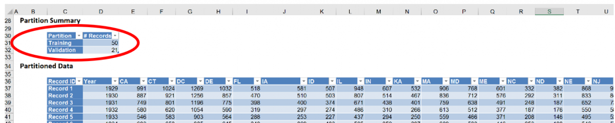
Note in the output above, the partitioning method is sequential (rather than random). The first 50 observations have been assigned to the training set and the remaining 21 observations have been assigned to the validation set.
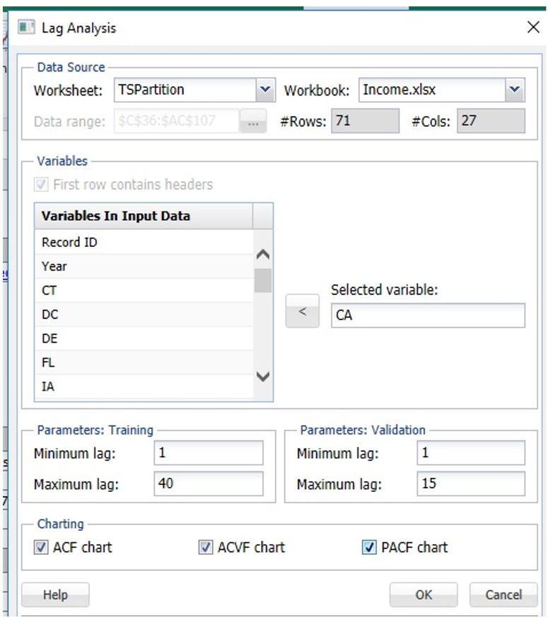
Open the Lag Analysis dialog by clicking ARIMA – Lag Analysis. Select CA under Variables in input data, then click > to move the variable to Selected variable. Enter 1 for Minimum Lag and 40 for Maximum Lag under Parameters: Training and 1 for Minimum Lag and 15 for Maximum Lag under Parameters: Validation.
Under Charting, select ACF chart, ACVF chart, and PACF chart to include each chart in the output.
Click OK. TS_Lags is inserted right of the TSPartition worksheet.
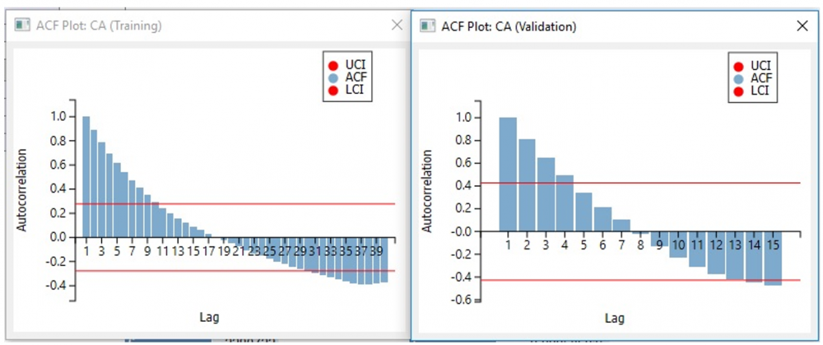
First, let's take a look at the ACF charts. Note on each chart, the autocorrelation decreases as the number of lags increase. This suggests that a definite pattern does exist in each partition. However, since the pattern does not repeat, it can be assumed that no seasonality is included in the data. In addition, both charts appear to exhibit a similar pattern.
Note: To view these two charts in the Cloud app, click the Charts icon on the Ribbon, select TS_Lags for Worksheet and ACF/ACVF/PACF Training/Validation Data for Chart.
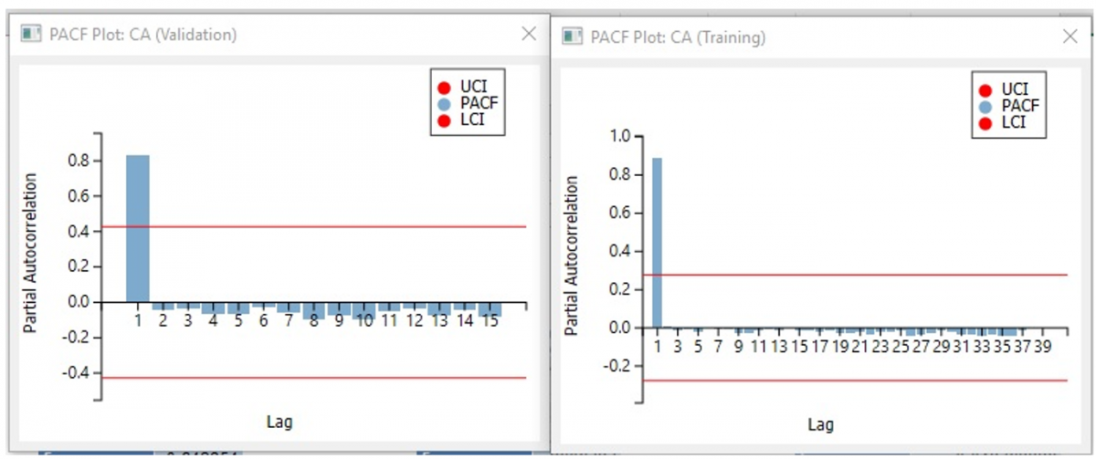
The PACF functions show a definite pattern which means there is a trend in the data. However, since the pattern does not repeat, we can conclude that the data does not show any seasonality.
The screenshots below display the autocovariance values.
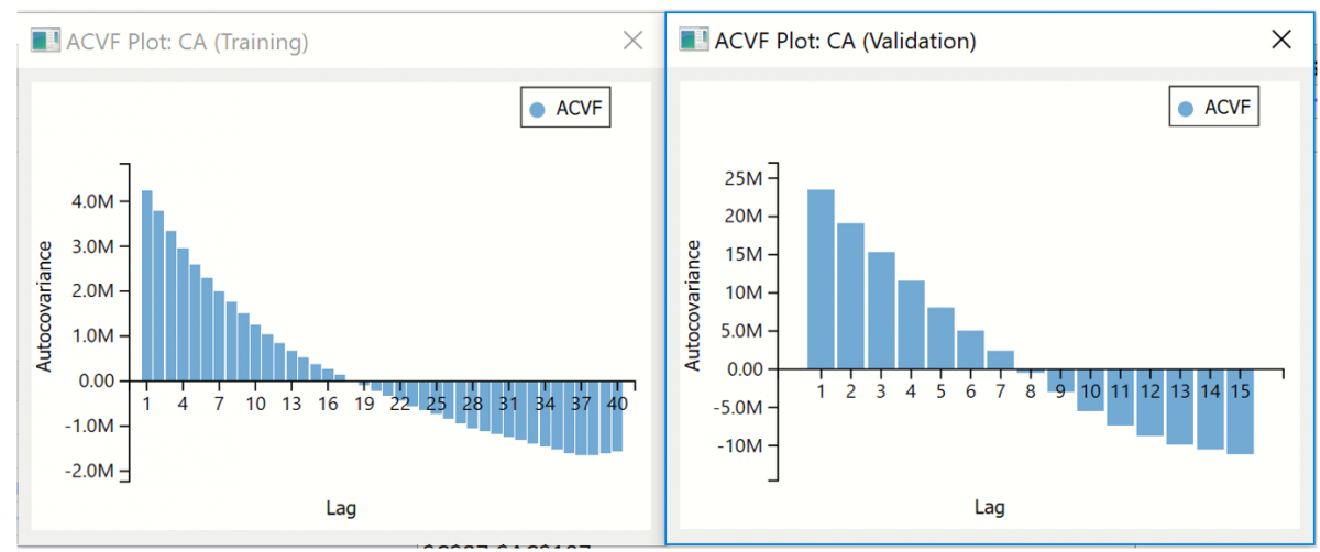
All three charts suggest that a definite pattern exists in the data, but no seasonality. In addition, both datasets exhibit the same behavior in both the training and validation sets which suggests that the same model could be appropriate for each. Now we are ready to fit the model.
The ARIMA model accepts three parameters: p – the number of autoregressive terms, d – the number of non-seasonal differences, and q – the number of lagged errors (moving averages).
Recall that the ACF plot showed no seasonality in the data which means that autocorrelation is almost static, decreasing with the number of lags increasing. This suggests setting q = 0 since there appears to be no lagged errors. The PACF plot displayed a large value for the first lag but minimal plots for successive lags. This suggest setting p =1. With most datasets, setting d =1 is sufficient or can at least be a starting point.
Click back to the TSPartition tab and then click ARIMA – ARIMA Model to bring up the Time Series – ARIMA dialog.
Select CA under Variables in input data then click > to move the variable to the Selected Variable field. Under Nonseasonal Parameters set Autoregressive (p) to 1, Difference (d) to 1 and Moving Average (q) to 0.
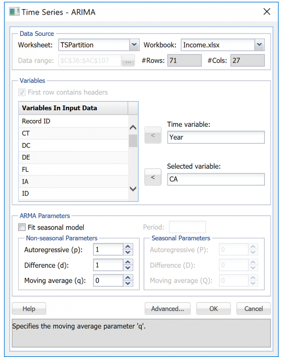
Click Advanced to open the ARIMA – Advanced Options dialog. Select Fitted Values and residuals, Produce forecasts, and Report Forecast Confidence Intervals. The default Confidence Level setting of 95 is automatically entered. The option Variance-covariance matrix is selected by default.

Click OK on the ARIMA-Advanced Options dialog and again on the Time Series – ARIMA dialog. Analytic Solver Data Science calculates and displays various parameters and charts in four output sheets, Arima_Output, Arima_Fitted, Arima_Forecast and Arima_Stored. Click the Arima_Output tab to view the Output Navigator.
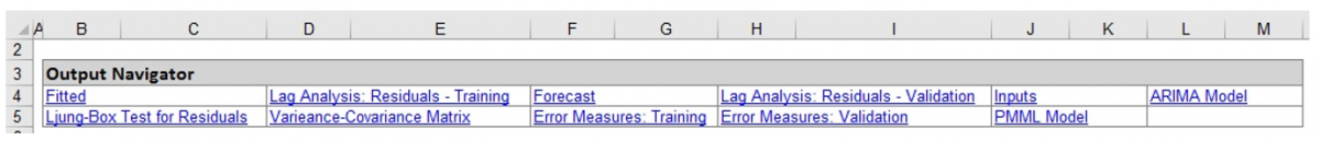
Click the ARIMA Model link on the Output Navigator to move to display the ARIMA Model and Ljung-Box Test Results on Residuals.
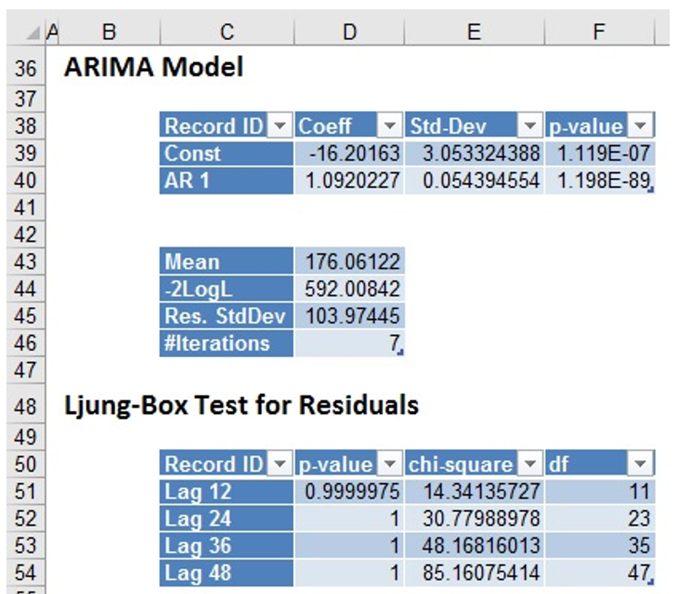
Analytic Solver has calculated the constant term and the AR1 term for our model, as seen above. These are the constant and f1 terms of our forecasting equation. See the following output of the Chi - square test.
The very small p-values for the constant term (1.119E-7) and AR1 term (1.19e-89) suggest that the model is a good fit to our data.
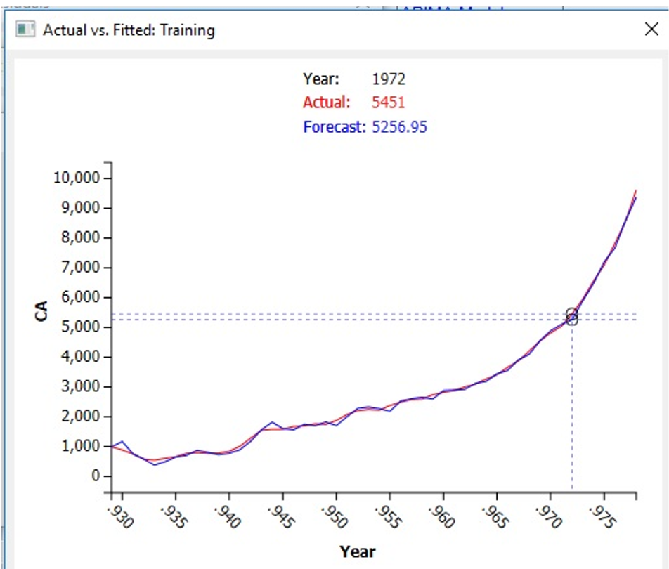
Click the Fitted link on the Output Navigator. This table plots the actual and fitted values and the resulting residuals for the training partition. As shown in the graph below, the Actual and Forecasted values match up fairly well. The usefulness of the model in forecasting will depend upon how close the actual and forecasted values are in the Forecast, which we will inspect later.
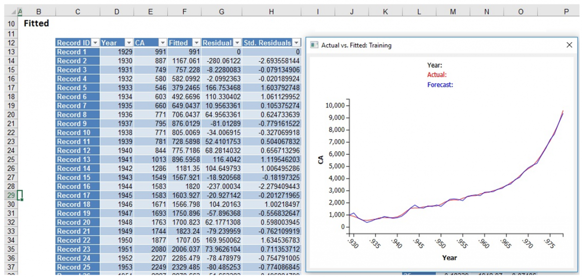
Use your mouse to select a point on the graph to compare the Actual value to the Forecasted value.
Note: To view these two charts in the Cloud app, click the Charts icon on the Ribbon, select Arima_Fitted for Worksheet and ACF/ACVF/PACF Training/Validation Data for Chart.
Take a look at the ACF and PACF plots for Errors found at the bottom of ARIMA_Output. Analytic Solver contains one more additional chart, the ACVF Plot for the Residuals.
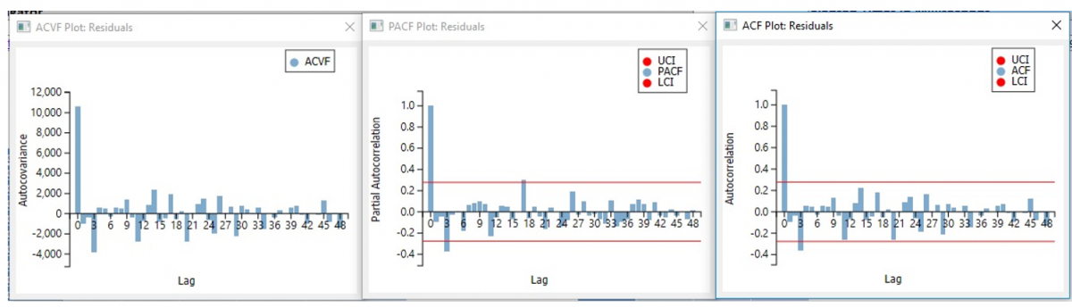
With the exception of Lag1, the majority of the lags in the PACF and ACF charts are either clearly within the UCL and LCL bands or just outside of these bands. This suggests that the residuals are random and are not correlated.
Click the Forecast link on the Output Navigator to display the Forecast Data table and charts.
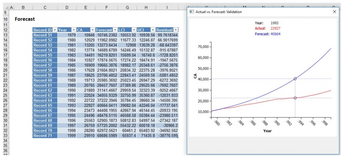
The table shows the actual and forecasted values along with LCI (Lower Confidence Interval), UCI (Upper Confidence Interval) and Residual values. The "Lower" and "Upper" values represent the lower and upper bounds of the confidence interval. There is a 95% chance that the forecasted value will fall into this range. The graph to the right plots the Actual values for CA against the Forecasted values. Again, click any point on either curve to compare the Actual against the Forecasted values.