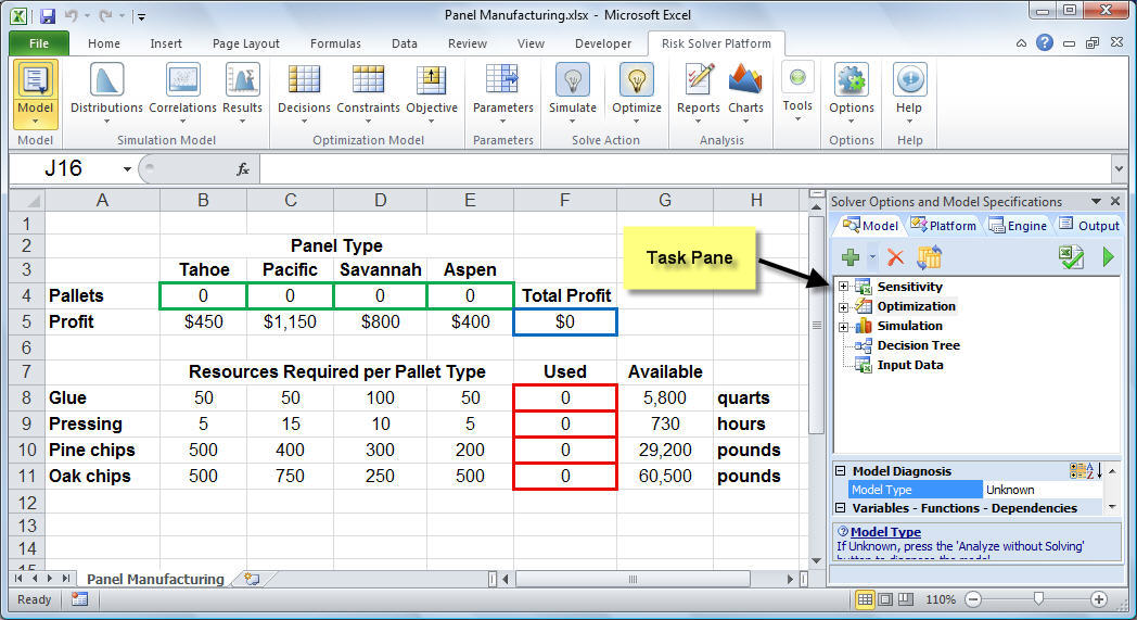
To let the Solver know which cells on the worksheet represent the decision variables, constraints and objective function, we click the Analytic Solver tab on the ribbon, which displays the icons shown below. (Click on the worksheet for a full-size image.) The Model icon on the Analytic Solver tab can be clicked to toggle on and off the Analytic Solver task pane shown on the right side of the screen.
To define the decision variables we select B4:E4 and then click Decisions, Normal on the Analytic Solver tab. Similarly, to define the objective, we select cell F5 and click Objective, Max, Normal on the Analytic Solver tab. The result of these settings are shown in the following worksheet. (Click the worksheet for a full-size image.)
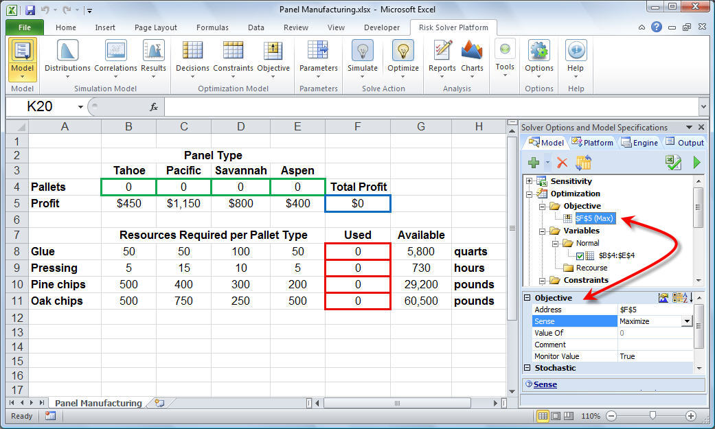
Notice that the Optimization icon in the task pane has expanded and is summarizing our selections for the objective and decision variables. Also notice that if we click on the objective cell in the task pane, various properties associated with the objective appear in the lower portion of the task pane. These properties allow us to change the cell to optimize and the direction of optimization (i.e., maximize or minimize). Similarly, if we click on the variables in the task pane, various properties associated with the variables would appear in the bottom of the task pane.
To add the constraints for the problem, we select cells F8:F11 and click Constraints, Normal Constraint, "<=" on the Analytic Solver tab. This causes the Add Constraint dialog to appear as shown below with cells F8:F11 in the Cell Reference edit box (the left hand side), and we select cells G8:G11 in the Constraint edit box (the right hand side). (Click on the worksheet to see a full-size image.)
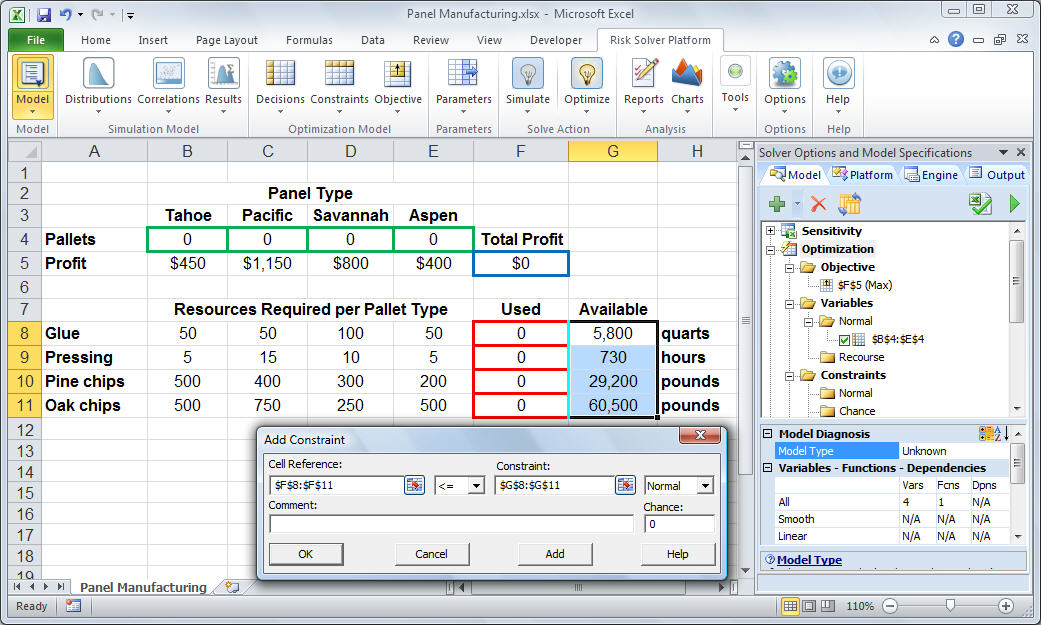
We can click the Add button on the Add Constraint dialog above (or click Constraints, Normal Constraints, ">=" on the Analytic Solver tab) to define the non-negativity constraints on the decision variables. (Alternatively, we can set the Assume Non-Negative property to True on the Engine tab in the task pane.)
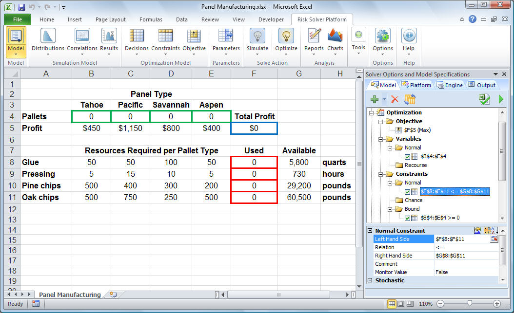
When we've completely entered the problem, the Analytic Solver task pane appears as shown below. (Click on the worksheet to see a full-size image.)
Finding and Using the Solution
To find the optimal solution, we simply click the Optimize icon on the Analytic Solver task pane (or the green triangular run/play button in the task pane). After a moment, the Solver returns the optimal solution in cells B4 through E4. This means that we should build 23 pallets of Tahoe panels, 15 pallets of Pacific panels, 39 pallets of Savannah panels, and 0 pallets of Aspen panels. This results in a total profit of $58,800 (shown in cell F5).
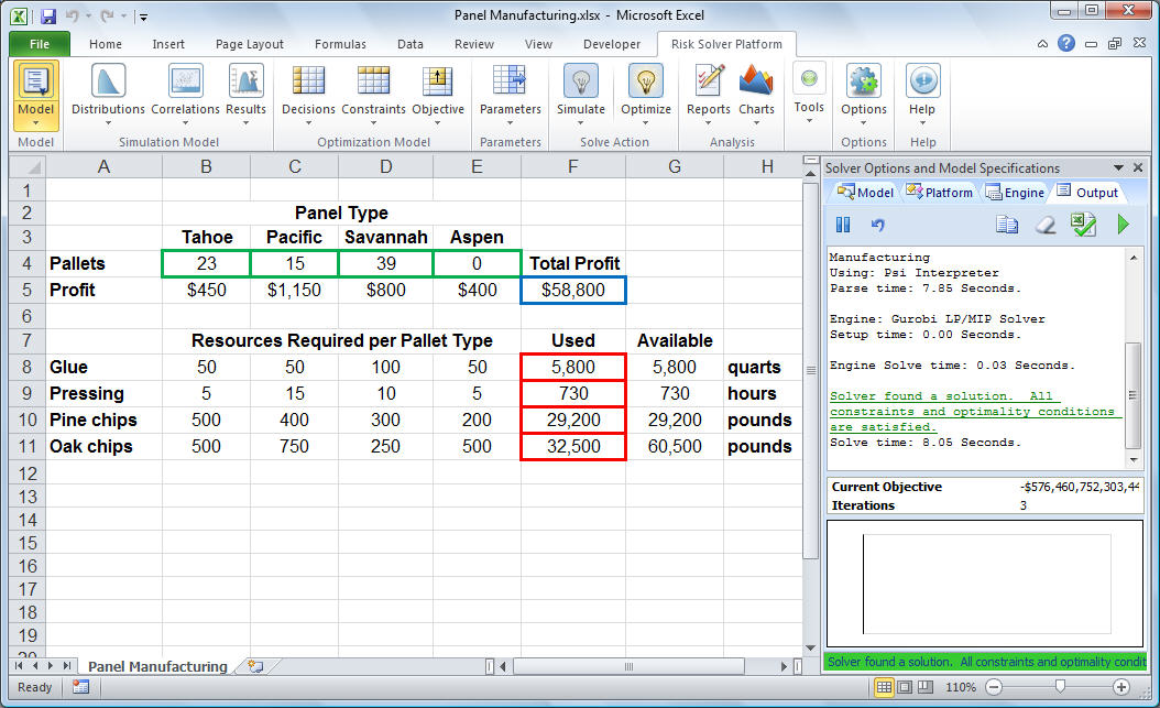
The message "Solver found a solution. All constraints and optimality conditions are satisfied." appears in the task pane, as shown above. (Click on the image to see it full-size). We now click Reports, Optimization, Answer in the Analytic Solver tab to produce an Answer Report. Analytic Solver creates another worksheet containing an Answer Report, like the one below, and inserts it to the left of the problem worksheet in the Excel workbook. (Click on the Answer Report for a full size image.)
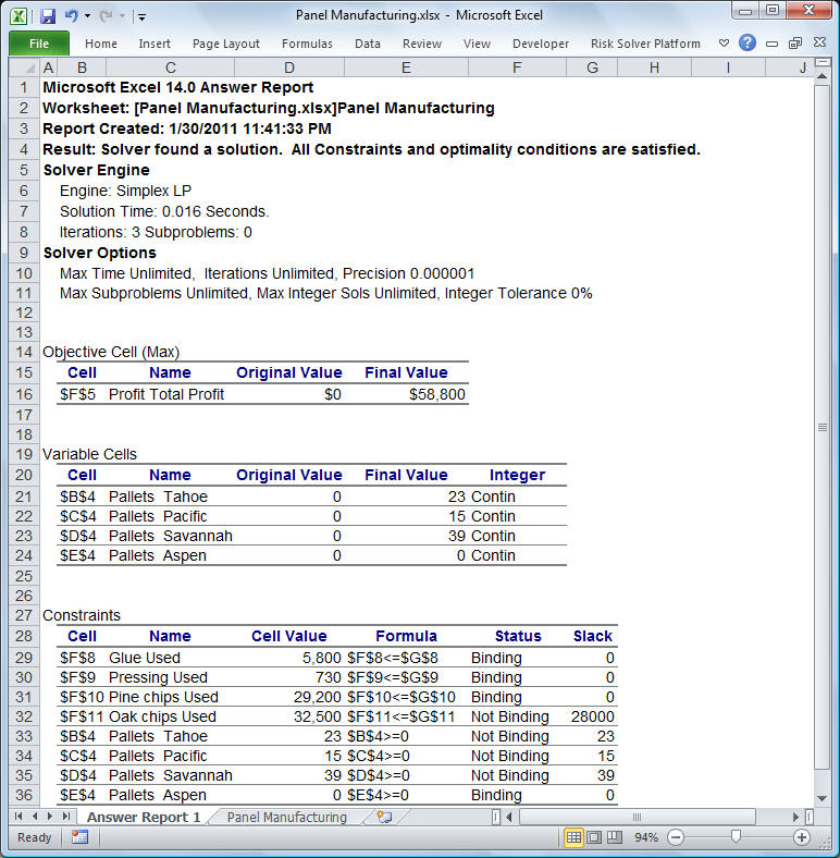
This report shows the original and final values of the objective function and the decision variables, as well as the status of each constraint at the optimal solution. Notice that the constraints on glue, pressing, and pine chips are binding and have a slack value of 0. The optimal solution would use up all of these resources; however, there were 28,000 pounds of oak chips left over. If we could obtain additional glue, pressing capacity, or pine chips we could further increase total profits, but extra oak chips would not help in the short run.
Learning More
If you've gotten to this point, congratulations! You've successfully set up and solved a simple optimization problem using Microsoft Excel. If you'd like, you can see how to set up and solve the same Product Mix problem using Excel's built-in Solver or using a Visual Basic .NET program that calls Frontline's Solver Platform SDK. If you haven't yet read the other parts of the tutorial, you may want to return to the Tutorial Start and read the overviews "What are Solvers Good For?", "How Do I Define a Model?", "What Kind of Solution Can I Expect?" and "What Makes a Model Hard to Solve?"
This was an example of a linear programming problem. Other types of optimization problems may involve quadratic programming, mixed-integer programming, constraint programming, smooth nonlinear optimization, and nonsmooth optimization. To learn more, click Optimization Problem Types. For a more advanced explanation of linearity and sparsity in optimization problems, continue with our Advanced Tutorial.