Introduction
Artificial neural networks are relatively crude electronic networks of neurons based on the neural structure of the brain. They process records one at a time, and learn by comparing their prediction of the record (largely arbitrary) with the known actual record. The errors from the initial prediction of the first record is fed back to the network and used to modify the network's algorithm for the second iteration. These steps are repeated multiple times.
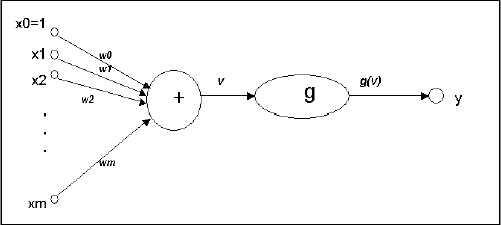
A neuron in an artificial neural network is:
1. A set of input values (xi) with associated weights (wi)
2. A input function (g) that sums the weights and maps the results to an output function(y).

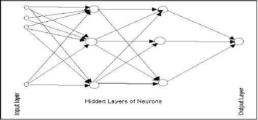
Neurons are organized into the following layers: input, hidden, and output. The input layer is composed not of full neurons, but simply of the values in a record that are inputs to the next layer of neurons. The next layer is the hidden layer of which there could be several. The final layer is the output layer, where there is one node for each class. A single sweep forward through the network results in the assignment of a value to each output node. The record is assigned to the class node with the highest value.

Training an Artificial Neural Network
In the training phase, the correct class for each record is known (i.e., supervised training), and the output nodes can be assigned correct values -- 1 for the node corresponding to the correct class, and 0 for the others. Results have been found using values of 0.9 and 0.1, respectively. As a result, it is possible to compare the network's calculated values for the output nodes to these correct values, and calculate an error term for each node. These error terms are then used to adjust the weights in the hidden layers so that the next time around the output values will be closer to the correct values.
The Iterative Learning Process
A key feature of neural networks is an iterative learning process in which records (rows) are presented to the network one at a time, and the weights associated with the input values are adjusted each time. After all cases are presented, the process often starts over again. During this learning phase, the network trains by adjusting the weights to predict the correct class label of input samples. Advantages of neural networks include their high tolerance to noisy data, as well as their ability to classify patterns on which they have not been trained. The most popular neural network algorithm is the back-propagation algorithm proposed in the 1980s.
Once a network has been structured for a particular application, that network is ready to be trained. To start this process, the initial weights are chosen randomly. Next, the training begins.
The network processes the records in the training data one at a time -- using the weights and functions in the hidden layers -- then compares the resulting outputs against the desired outputs. Errors are then propagated back through the system, causing the system to adjust the weights for the next record. This process occurs again as the weights are continually tweaked. During the training of a network, the same set of data is processed many times as the connection weights are continually refined.
Note that some networks never learn. This could be because the input data does not contain the specific information from which the desired output is derived. Networks also will not converge if there is not enough data to enable complete learning. Ideally, there should be enough data available to create a Validation Set.
Feedforward, Back-Propagation
The feedforward, back-propagation architecture was developed in the early 1970s by several independent sources (Werbor, Parker, Rumelhart, Hinton, and Williams). This independent co-development was the result of a proliferation of articles and talks at various conferences that stimulated the entire industry. Currently, this synergistically developed back-propagation architecture is the most popular and effective model for complex, multi-layered networks. Its greatest strength is in non-linear solutions to ill-defined problems. The typical back-propagation network has an input layer, an output layer, and at least one hidden layer. Theoretically, there is no limit on the number of hidden layers, but typically there are just one or two. Some studies have shown that the total number of layers needed to solve problems of any complexity is five (one input layer, three hidden layers, and an output layer). Each layer is fully connected to the succeeding layer.
The training process normally uses some variant of the Delta Rule, which starts with the calculated difference between the actual outputs and the desired outputs. Using this error, connection weights are increased in proportion to the error times, which are a scaling factor for global accuracy. This means that the inputs, the output, and the desired output all must be present at the same processing element. The most complex part of this algorithm is determining which input contributed the most to an incorrect output and how to modify the input to correct the error. (An inactive node would not contribute to the error and would have no need to change its weights.) To solve this problem, training inputs are applied to the input layer of the network, and desired outputs are compared at the output layer. During the learning process, a forward sweep is made through the network, and the output of each element is computed layer by layer. The difference between the output of the final layer and the desired output is back-propagated to the previous layer(s), usually modified by the derivative of the transfer function. The connection weights are normally adjusted using the Delta Rule. This process proceeds for the previous layer(s) until the input layer is reached.
Structuring the Network
The number of layers and the number of processing elements per layer are important decisions. To a feedforward, these parameters back-propagation topology, are also the most ethereal - they are the art of the network designer. There is no quantifiable, best answer to the layout of the network for any particular application. There are only three general rules picked up over time and followed by most researchers and engineers applying this architecture to their problems.
Ensemble Methods
Analytic Solver Data Science offers two powerful ensemble methods for use with Neural Networks: bagging (bootstrap aggregating) and boosting. The Neural Networks Algorithm on its own can be used to find one model that results in good predictions for the new data. We can view the statistics and confusion matrices of the current predictor to see if our model is a good fit to the data, but how would we know if there is a better predictor just waiting to be found? The answer is that we do not know if a better predictor exists. However, ensemble methods allow us to combine multiple weak neural networks which, when taken together form a new, more accurate strong neural networks. These methods work by creating multiple diverse networks, by taking different samples of the original dataset, and then combining their outputs. (Outputs may be combined by several techniques for example, majority vote for classification and averaging for prediction.) This combination of models effectively reduces the variance in the strong model. The two different types of ensemble methods offered in Analytic Solver Data Science (bagging and boosting) differ on three items: 1) the selection of training data for each predictor or weak model; 2) how the weak models are generated; and 3) how the outputs are combined. In all three methods, each weak model is trained on the entire Training Set to become proficient in some portion of the data set.
Bagging (bootstrap aggregating) was one of the first ensemble algorithms written. Bagging generates several Training Sets by using random sampling with replacement (bootstrap sampling), applies the neural network algorithm to each data set, then takes the average among the models to calculate the predictions for the new data. The biggest advantage of bagging is the relative ease that the algorithm can be parallelized, which makes it a better selection for very large data sets.
Boosting builds a strong model by successively training models to concentrate on records receiving inaccurate predicted values in previous models. Once completed, all predictors are combined by a weighted majority vote. Analytic Solver Data Science offers three different variations of boosting as implemented by the AdaBoost algorithm (one of the most popular ensemble algorithms in use today): M1 (Freund), M1 (Breiman), and SAMME (Stagewise Additive Modeling using a Multi-class Exponential).
Adaboost.M1 first assigns a weight (wb(i)) to each record or observation. This weight is originally set to 1/n, and will be updated on each iteration of the algorithm. An original neural network is created using this first training set (Tb) and an error is calculated as:

where, the I() function returns 1 if true and 0 if not.
The error of the network in the bth iteration is used to calculate the constant αb. This constant is used to update the weight wb(i). In AdaBoost.M1 (Freund), the constant is calculated as
αb= ln((1-eb)/eb)
In AdaBoost.M1 (Breiman), the constant is calculated as
αb= 1/2ln((1-eb)/eb)
In SAMME, the constant is calculated as
αb= 1/2ln((1-eb)/eb + ln(k-1) where k is the number of classes
where, the number of categories is equal to 2, SAMME behaves the same as AdaBoost Breiman.
In any of the three implementations (Freund, Breiman, or SAMME), the new weight for the (b + 1)th iteration will be

Afterwards, the weights are all readjusted to sum to 1. As a result, the weights assigned to the observations that were assigned inaccurate predicted values are increased, and the weights assigned to the observations that were assigned accurate predicted values are decreased. This adjustment forces the next neural network to put more emphasis on the records that were assigned inaccurate predictions. (This constant is also used in the final calculation, which will give the network with the lowest error more influence.) This process repeats until b = Number of weak learners (controlled by the User). The algorithm then computes the weighted average among all weak learners and assigns that value to the record. Boosting generally yields better models than bagging, however, it does have a disadvantage as it is not parallelizable. As a result, if the number of weak learners is large, boosting would not be suitable.
Neural Network Ensemble methods are very powerful methods and typically result in better performance than a single network. This feature addition in Analytic Solver Data Science provides users with more accurate prediction models, and should be considered over the single network method.
