The example below illustrates the use of Analytic Solver Data Science’s chart wizard in drawing a histogram of the Utilities dataset. Click Help – Example Models on the Data Science ribbon to open the example dataset, Utilities.xlsx under Forecasting/Data Science Example Models. Select a cell within the dataset, say A2, and then click Explore – Chart Wizard on the Data Science ribbon. Select Histogram, and then click Next.
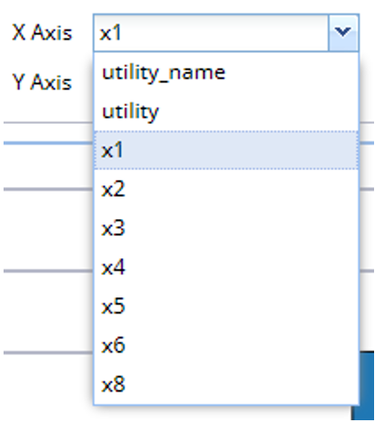
On the opening chart, select X1 for the X Axis to create a histogram of the values for the x1 variable.
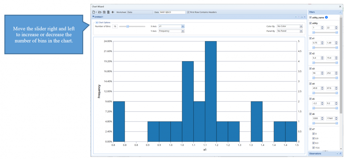
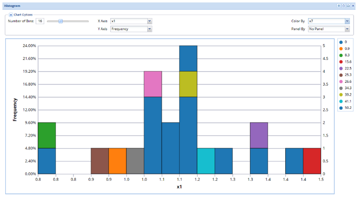
Move the slider right and left to increase or decrease the number of bins in the chart.
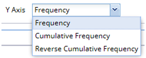
For the Y Axis, select Frequency, Cumulative Frequency or Reverse Cumulative Frequency.
Set Color By to x7. This new chart indicates the corresponding value for x7 for each utility. For example, the 5th bin consists of 1 value, 0.96 for the Pacific utility. The color of this bin indicates that the value of x7 for this specific utility is 0.9.
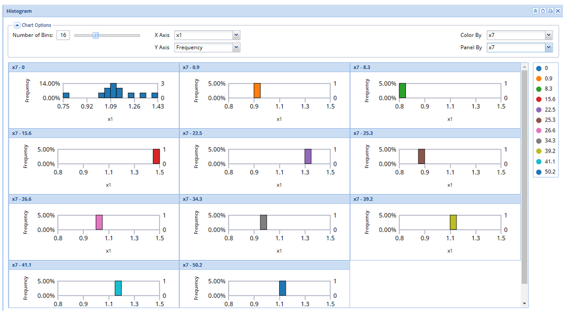
Set Panel by to X7. This chart creates 11 different graphs; one graph for each of the values for x7: 0, 0.9, 8.3, 15.6, 22.5, 25.3, 26.6, 34.3, 39.2, 41.1, 50.2. Notice that labels for each of the graphs, i.e. x7-0, x7-0.9, x7 – 8.3, etc. Each chart plots the corresponding value for the x1 variable, for example the SanDiego utility has a value of 8.3 for x7. The value for x1 (0.76) is plotted in the x7-8.3 chart.