This example illustrates how to use Analytic Solver’s Double Exponential Smoothing technique to uncover seasonality trends in the Airpass.xlsx time series dataset. (See the examples above for instructions on how to open this example.)
Click Partition in the Time Series group on the Data Science ribbon to open the Time Series Partition dialog. Select Month as the Time Variable. Select Passengers as the Variables in the Partition Data.

Then click OK to partition the data into training and validation sets. TSPartition will be inserted right of the Airpass worksheet.
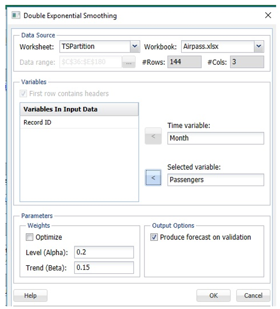
Click Smoothing – Double Exponential to open the Double Exponential Smoothing dialog.
Select Month as the Time Variable, if not already selected. Select Passengers as the Selected variable, then check Produce Forecast on validation to test the forecast on the validation set.
This example uses the defaults for both the Alpha and Trend parameters. However, Analytic Solver Data Science includes a feature that will choose the Alpha and Trend parameter values that result in the minimum residual mean squared error. It is recommended that this feature be used carefully as this feature most often leads to a model that is overfit to the training set. An overfit model rarely exhibits high predictive accuracy in the validation set.
Click OK to run the Double Exponential Smoothing algorithm. The output, DoubleExpo and DoubleExpo_Stored, will be inserted right of the TSPartition worksheet.
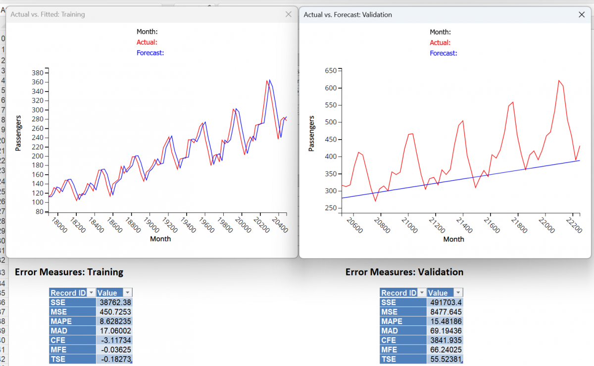
Click on the DoubleExpo tab to view the results of the smoothing. Click on any point on either graph to see the Actual vs. Forecast results at the top of the chart.
Note: To view these two charts in the Cloud app, click the Charts icon on the Ribbon, select DoubleExp for Worksheet and Time Series Training Data or Time Series Validation Data for Chart.

If instead, the Optimize feature is used ….

... an Alpha of 0.9568 is chosen along with a Trend of 0.009.

These parameters result in a MSE of 450.7 for the Training set and a MSE of 8477.64 for the Validation Set. Again the model created with the parameters from the Optimize algorithm appear to result in a model with a better fit than a model created with the default parameters.
Note: To view these two charts in the Cloud app, click the Charts icon on the Ribbon, select DoubleExp1 for Worksheet and Time Series Training Data or Time Series Validation Data for Chart.