When data collected over time displays random variation, smoothing techniques can be used to reduce or cancel the effect of these variations. When properly applied, these techniques smooth out the random variation in the time series data to reveal underlying trends.
Analytic Solver Data Science features four different smoothing techniques: Exponential, Moving Average, Double Exponential, and Holt-Winters. Exponential and Moving Average are relatively simple smoothing techniques and should not be performed on data sets involving seasonality. Double Exponential and Holt-Winters are more advanced techniques that can be used on data sets involving seasonality.
Exponential Smoothing
Exponential Smoothing is one of the more popular smoothing techniques due to its flexibility, ease in calculation, and good performance. Exponential Smoothing uses a simple average calculation to assign exponentially decreasing weights starting with the most recent observations. New observations are given relatively more weight in the average calculation than older observations. The Exponential Smoothing tool uses the following formulas.
S0= x0
St = αxt-1 + (1-α)st-1, t > 0
where
- original observations are denoted by {xt} starting at t = 0
- α is the smoothing factor which lies between 0 and 1
Exponential Smoothing should only be used when the data set contains no seasonality. The forecast is a constant value that is the smoothed value of the last observation.
Moving Average Smoothing
In Moving Average Smoothing, each observation is assigned an equal weight, and each observation is forecasted by using the average of the previous observation(s). Using the time series X1, X2, X3, ....., Xt, this smoothing technique predicts Xt+k as follows :
St = Average (xt-k+1, xt-k+2, ....., xt), t= k, k+1, k+2, ...N
where k is the smoothing parameter.
Analytic Solver Data Science allows a parameter value between 2 and t-1 where t is the number of observations in the data set. Note that when choosing this parameter, a large parameter value will oversmooth the data, while a small parameter value will undersmooth the data. The past three observations will predict the future observations. As with Exponential Smoothing, this technique should not be applied when seasonality is present in the data set.
Double Exponential Smoothing
Double Exponential Smoothing can be defined as the recursive application of an exponential filter twice in a time series. Double Exponential Smoothing should not be used when the data includes seasonality. This technique introduces a second equation that includes a trend parameter; thus, this technique should be used when a trend is inherent in the data set, but not used when seasonality is present. Double Exponential Smoothing is defined by the following formulas.
St = At + Bt , t = 1,2,3,..., N
Where, At = axt + (1- a) St-1 0< a <= 1
Bt = b (At - At-1) + (1 - b ) Bt-1 0< b <= 1
The forecast equation is: Xt+k = At + K Bt , K = 1, 2, 3, ...
where, a denotes the Alpha parameter, and b denotes the trend parameters. These two parameters can be entered manually.
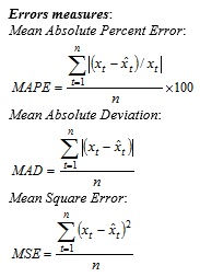
Analytic Solver Data Science includes an optimize feature that will choose the best values for alpha and trend parameters based on the Forecasting Mean Squared Error. If the trend parameter is 0, then this technique is equivalent to the Exponential Smoothing technique. (However, results may not be identical due to different initialization methods for these two techniques.)
Holt-Winters Smoothing
Holt Winters Smoothing introduces a third parameter (g) to account for seasonality (or periodicity) in a data set. The resulting set of equations is called the Holt-Winters method, after the names of the inventors. The Holt-Winters method can be used on data sets involving trend and seasonality (a, b , g). Values for all three parameters can range between 0 and 1.
The following three models associated with this method.
Multiplicative: Xt = (At+ Bt)* St +et where At and Bt are previously calculated initial estimates. St is the average seasonal factor for the tth season.
At = axt/St-p + (1-a)(At-1 + Bt-1)
Bt = b(At + At-1) + (1 - b)Bt-1
St = gxt/At + (1 - g)St-p
Additive: Xt = (At+ Bt) +St + et
No Trend: b = 0, so, Xt = A * St +et

Holt-Winters smoothing is similar to Exponential Smoothing if b and g = 0, and is similar to Double Exponential Smoothing if g = 0.
