Fixed # Components Example

This example uses a fixed number of components in the ‘reduced’ model. 

Click Transform – Principal Components on the Data Science ribbon to open the Principal Components Analysis dialog.  On the Data tab, select variables x1 to x8, then click the > command button to move them to the Selected Variables field.

Click Next to move to the Parameters tab. 

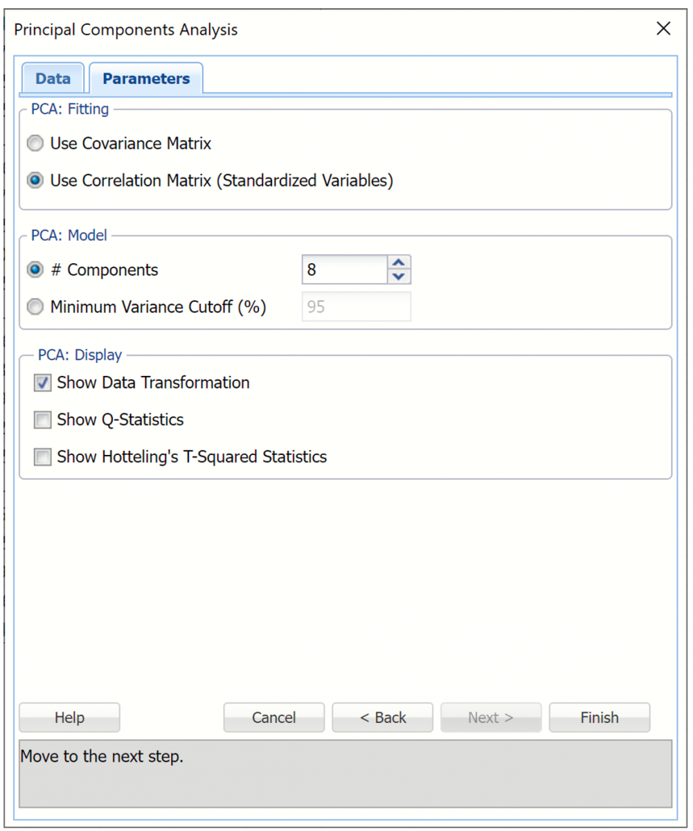
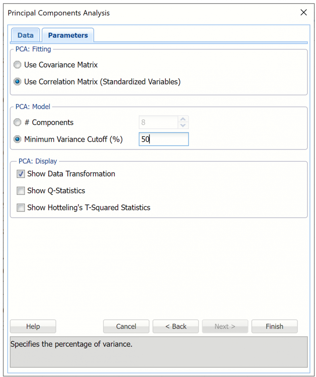
Analytic Solver Data Science provides two routines for specifying the number of principal components in the model: # Components and Minimum Variance Cutoff. 

• The # Components (the default) method allows the user to specify a fixed number of components, or variables, to be included in the “reduced” model.  The default setting for this option is equal to the number of selected variables.  This value can be decreased to 1.    
• The Minimum Variance Cutoff method allows the user to specify a percentage of the variance.  When this method is selected, Analytic Solver Data Science will calculate the minimum number of principal components required to account for that percentage of the variance.

In addition, Analytic Solver Data Science provides two methods for calculating the principal components:  using the covariance or the correlation matrix. 

When using the correlation matrix method, the data will be normalized first before the method is applied.  (The dataset is normalized by dividing each variable by its standard deviation.)  Normalizing gives all variables equal importance in terms of variability.  If the covariance method is selected, the dataset should first be normalized.  Note:  The Correlation Matrix is used only for internal calculations and is not included in the output results. 

Under PCA:  Display, confirm Show Data Transformation is selected by default.  This option displays an output matrix where the columns are the principal components, the rows are the individual data records and the value in each cell is the calculated score for that record on the relevant principal component. 

For a description of Show Q-Statistics and Show Hotteling's T-Squared Statistics options, please see the Principal Components Options section below.

Click Finish to run PCA. 

 

PCA Output Worksheets

Two worksheets are inserted to the right of the Data worksheet:  PCA_Output and PCA_Scores. PCA_Output contains the Inputs, the Principal Components table and the Explained Variance table.  PCA_Scores contains the Scores table. 

Click the PCA_Output tab. The inputs table is shown below.  This table displays the options selected on both tabs of the Principal Components Analysis dialog. 

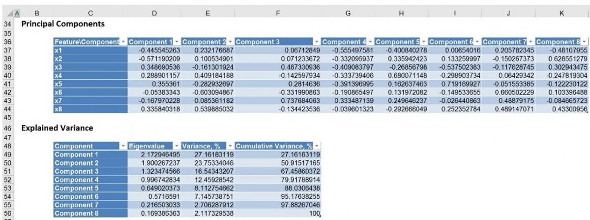
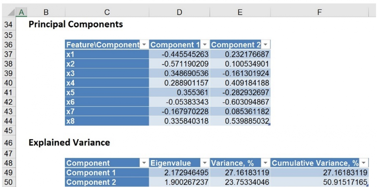
Further down the PCA_Output worksheet is the Principal Components table.  The maximum magnitude element for Component1 corresponds to x2 (-0.5712).  This signifies that the first principal component is measuring the effect of x2 on the utility companies.  Likewise, the second component appears to be measuring the effect of x6 on the utility companies (maximum magnitude = |-0.6031|). 

Take a look at the Explained Variance table.  The Variance, % column displays Component1 as accounting for 27.16% of the variance while the second component accounts for 23.75%.  Together, these two components account for more than 50% of the total variation.  You can alternatively say the maximum magnitude element for component 1 corresponds to x2.

PCA_Scores

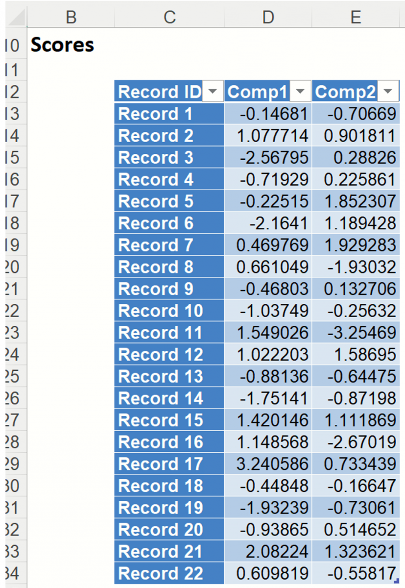
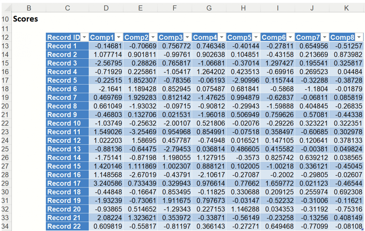
Double click PCA_Scores in the taskpane or click the PCA_Scores worksheet tab to view the Principal Components table.  This table holds the weighted averages of the normalized variables (after each variable’s mean is subtracted).  (This matrix is described in the 2nd step of the PCA algorithm - see Introduction above.) Again, we are looking for the magnitude or absolute value of each figure in the table. 

Minimum Variance Cutoff Example

The Minimum Variance Cutoff method allows the user to specify a percentage of the variance.  When this method is selected, Analytic Solver Data Science will calculate the minimum number of principal components required to account for that percentage of the variance.

Click back to the Data sheet, then reopen the Principal Components Analysis dialog.  Cells x1 through x8 are already selected.  Click Next on the dialog to advance to the Parameters tab.

This time, select Minimum Variance Cutoff and enter 50 for %.  Keep Use Correlation Matrix (Use Standardized Variables) and Show Data Transformation selected, then click Finish. 

Output Worksheets

Open PCA_Output1 and scroll down to the Principal Components and Explained Variance tables.  Notice that only the first two components are included in the output file since these two components account for over 50% of the variation. 

Note:  The Correlation Matrix is used only for internal calculations and is not included in the output results. 

The output from PCA_Scores1 is shown below.  This table holds the weighted averages of the normalized variables (after each variable’s mean is subtracted).  (This matrix is described in the 2nd step of the PCA algorithm - see Introduction above.) Again, we are looking for the magnitude or absolute value of each figure in the table.