Principal Component Analysis Options
below for an explanation of options on both tabs of the Principal Components Analysis (PCA) dialog: Data and Parameters.
The following options appear on all three tabs of the Principal Components Analysis dialog.

Help: Click the Help button to access documentation on all Principal Components Analysis options.
Cancel: Click the Cancel button to close the dialog without running Principal Components Analysis.
Next: Click the Next button to advance to the next tab.
Finish: Click Finish to accept all option settings on both dialogs, and run Principal Components Analysis.
Principal Components Analysis Data Tab
See below for documentation for all options appearing on the Data tab.
Principal Components Analysis Data Tab
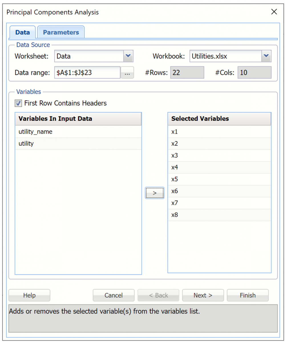
Data Source
Worksheet: Click the down arrow to select the desired worksheet where the dataset is contained.
Workbook: Click the down arrow to select the desired workbook where the dataset is contained.
Data range: Select or enter the desired data range within the dataset. This data range may either be a portion of the dataset or the complete dataset.
#Columns: Displays the number of columns in the data range. This option is read only.
#Rows: Displays the number of rows in the data range. This option is read only.
Variables
First Row Contains Headers: Select this checkbox if the first row in the dataset contains column headings.
Variables In Input Data: This field contains the list of the variables, or features, included in the data range.
Selected Variables: This field contains the list of variables, or features, to be included in PCA.
- To include a variable in PCA, select the variable in the Variables In Input Data list, then click > to move the variable to the Selected Variables list.
- To remove a variable as a selected variable, click the variable in the Selected Variables list, then click < to move the variable back to the Variables In Input Data list.
Principal Components Analysis Parameters Tab
See below for documentation for all options appearing on the Principal Components Analysis Parameters tab.
Principal Components Analysis, Parameters Tab
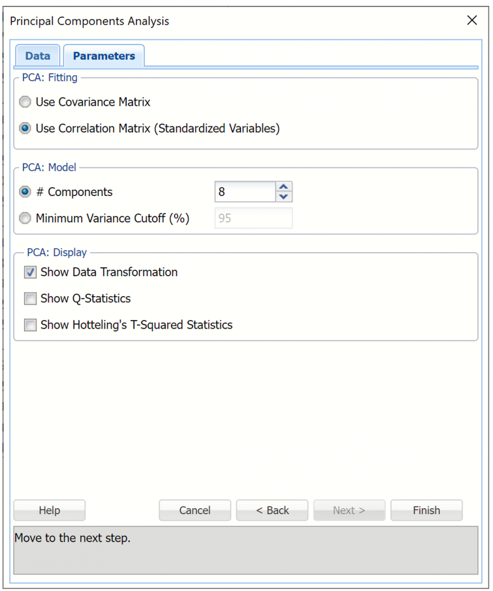
PCA: Fitting
To compute Principal Components the data is matrix multiplied by a transformation matrix. This option lets you specify the choice of calculating this transformation matrix.
Use Covariance matrix
The covariance matrix is a square, symmetric matrix of size n x n (number of variables by number of variables). The diagonal elements are variances and the off-diagonals are covariances. The eigenvalues and eigenvectors of the covariance matrix are computed and the transformation matrix is defined as the transpose of this eigenvector matrix. If the covariance method is selected, the dataset should first be normalized. One way to organize the data is to divide each variable by its standard deviation. Normalizing gives all variables equal importance in terms of variability.[1]
Use Correlation matrix (Standardized Variables)
An alternative method is to derive the transformation matrix on the eigenvectors of the correlation matrix instead of the covariance matrix. The correlation matrix is equivalent to a covariance matrix for the data where each variable has been standardized to zero mean and unit variance. This method tends to equalize the influence of each variable, inflating the influence of variables with relatively small variance and reducing the influence of variables with high variance. This option is selected by default.
PCA: Model
Select the number of principal components displayed in the output.
# components
Specify a fixed number of components by selecting this option and entering an integer value from 1 to n where n is the number of Input variables selected in the Data tab. This option is selected by default, the default value of n is equal to the number of input variables. This value can be decreased to 1.
Minimum Variance Cutoff (%)
Select this option to specify a percentage. Analytic Solver Data Science will calculate the minimum number of principal components required to account for that percentage of variance.
PCA: Display
Select the type of output to be inserted into the workbook in this section of the Parameters tab. If no output is selected, by default, PC will output three tables: Inputs, Principal components and Explained Variance on the PCA_Output worksheet.
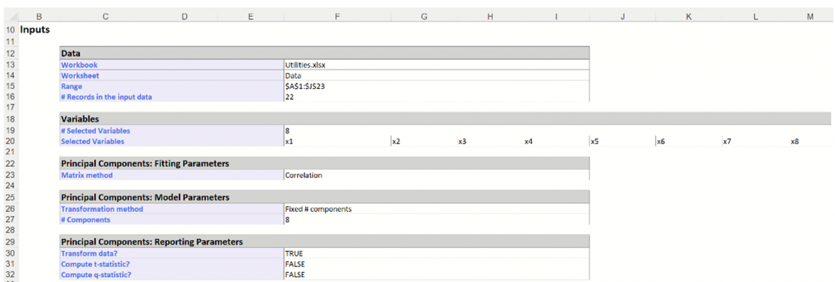
Inputs: This table displays the options selected on both tabs of the Principal Components Analysis dialog. This table is accessible by clicking the Inputs link in the Output Navigator.
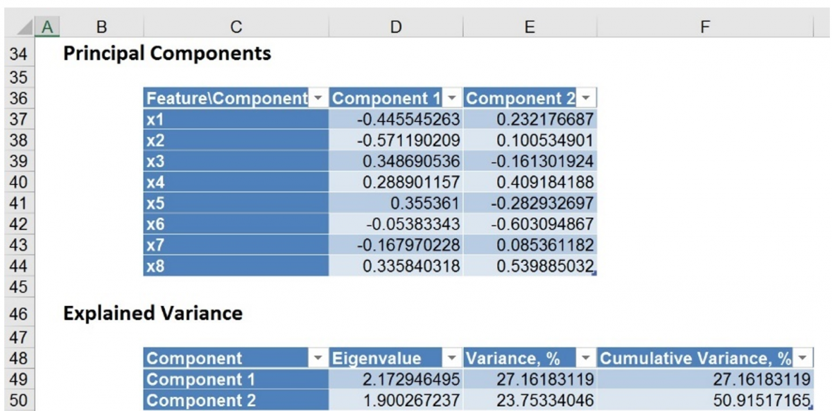
Principal Components: This table displays how each variable affects each component.
In the example below, the maximum magnitude element for Component1 corresponds to x2 (-0.5712). This signifies that the first principal component is measuring the effect of x2 on the utility companies. Likewise, the second component appears to be measuring the effect of x6 on the utility companies (maximum magnitude = |-0.6031|). This table is accessible by clicking the Principal Components link in the Output Navigator.
Explained Variance: This table includes 3 columns: Eigenvalue, Variance, % and Cumulative Variance. This table is accessible by clicking the Explained Variance link in the Output Navigator.
- The Eigenvalue column displays the eigenvalues and eigenvectors computed from the covariance matrix for each variable. They are listed in order from largest to smallest. Larger eigenvalues denote that the variable should remain in the database. Variables with smaller eigenvalues will be removed according to the user’s preference.
- The Variance, % column displays the variance attributed by each Component. In the example below, Component1 accounts for 27.16% of the variance while the second component accounts for 23.75%.
- The Cumulative Variance column displays the cumulative variance. In the example below, Components 1 and 2 account for more than 50% of the total variation. You can alternatively say the maximum magnitude element for component 1 corresponds to x2.
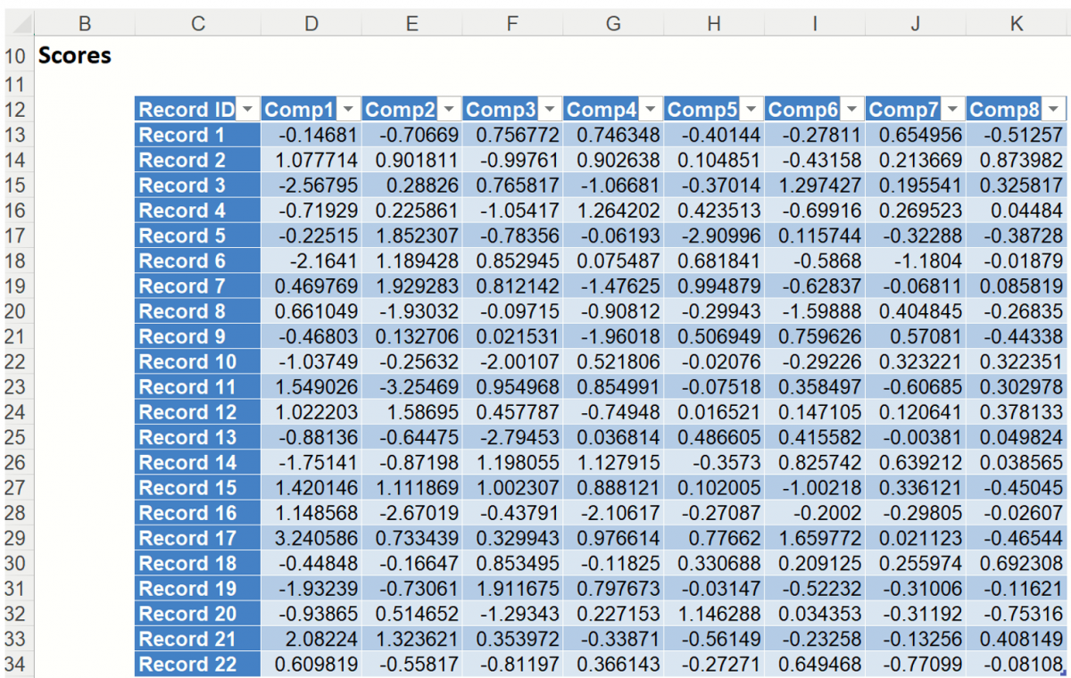
Show Data Transformation
This option results in the display of a matrix, Scores, in which the columns are the principal components, the rows are the individual data records, and the value in each cell is the calculated score for that record on the relevant principal component. This option is selected by default.
This table holds the weighted averages of the normalized variables (after each variable’s mean is subtracted). (This matrix is described in the 2nd step of the PCA algorithm - see Introduction above.) When reading the table, note the magnitude or absolute value of each value in the table. This table is accessible by clicking the Scores link in the Output Navigator.
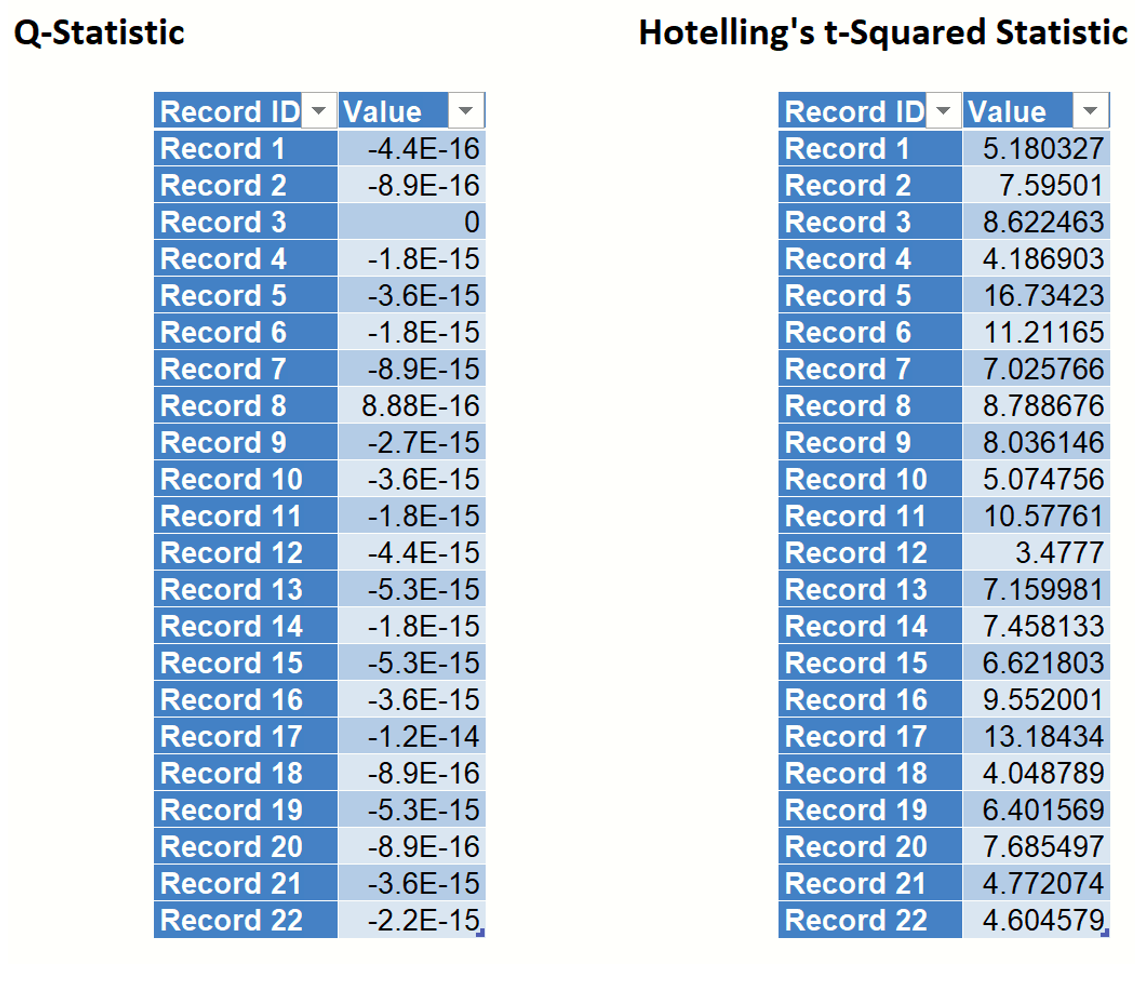
Q Statistics and Hotteling’s T-Squared Statistics
Q Statistics, or residuals, and Hotteling’s T-Squared statistics are summary statistics which help explain how well a model fits the sample data and can also be used to detect any outliers in the data. A detailed explanation for each is beyond the scope of this guide. Please see the literature for more information on each of these statistics.
Show Q - Statistics
If this option is selected, Analytic Solver Data Science will include Q-Statistics in the output worksheet, PCA_Stats. Q statistics (or residuals) measure the difference between sample data and the projection of the model onto the sample data. These statistics an also be used to determine if any outliers exist in the data. Low values for Q statistics indicate a well fit model. This table is also accessible by clicking the Q-Statistic link in the Output Navigator.
Show Hotteling’s T-Squared Statistics
If this option is selected, Analytic Solver Data Science will include Hotteling’s T-Squared statistics in the output worksheet, PCA_Stats. T-Squared statistics measure the variation in the sample data within the mode and indicate how far the sample data is from the center of the model. These statistics can also be used to detect outliers in the sample data. Low T-Squared statistics indicate a well fit model. This table is accessible by clicking the Hotteling’s t-Squared Statistic link in the Output Navigator.
[1] Shmueli, Galit, Nitin R. Patel, and Peter C. Bruce. Data Science for Business Intelligence. 2nd ed. New Jersey: Wiley, 2010